At the time of writing, the Royals are a disappointing 40-47. This performance is disappointing considering they won a playoff series last year. The culprit of the lackluster season is the offense: they have scored the fewest runs in all of Major League Baseball.
No one expected the Royals to have a top-10 offense. At the same time, this level of offensive struggle was certainly not expected. However, this point raises a research question: how unlikely is their offense performance? How surprised should we be by the actual statistics?
Likewise, one of the strikingly lackluster parts of the offense is how almost all individual players have underperformed expectations (with the exception of Maikel Garcia). Therefore, I wanted to center my analysis on the probability of individual players performing as they have this season. In other words, what is the probability of so many individual players underperforming in the same season?
The analysis assumes that player performance is independent, which is a fairly good but not perfect assumption. How Bobby Witt Jr. and Salvador Perez perform can influence one another, so can shared phenomena (e.g., team culture). That said, baseball stats display notable elements of independence. Maikel Garcia can have a great season even when Jonathan India struggles.
The OPS data for this analysis was pulled on 7/1/25. For the 9 Royals who have played the most games, I created what I deemed to be a reasonable expectation of their OPS along with a plausible standard deviation for the same metric. Surely, this process included some subjectivity, though I believe the figures to be realistic. Taking a purely statistical approach is difficult due to small sample sizes and the fact that player expectations change over time (we do not expect Salvy to hit like he did in 2021 when he smashed 48 home runs).
Therefore, some level of bias is likely creeping into the analysis. The biggest risk is in systemic bias: my level of subjectivity is not consistent across players. I have done my best to combat this pitfall, but this concern is still worth calling out. Additionally, these are not full-season results and, consequently, could be suffering from some statistical noise. That said, my goal is not to construct the perfect analysis but rather one that is useful and illustrative. I believe this work accomplishes those aims.
Below is the raw data. The actual_ops is the player’s performance until 7/1. The ops_expectation and ops_std are variables I synthesized based on each players’ historical data while making adjustments to capture a plausible “current expectation” for their 2025 performance.
| player | actual_ops | ops_expectation | ops_std |
| Salvador Perez | 656 | 740 | 60 |
| Vinnie Pasquantino | 738 | 760 | 60 |
| Bobby Witt Jr | 825 | 925 | 50 |
| Maikel Garcia | 846 | 700 | 50 |
| Jonathan India | 664 | 740 | 50 |
| Kyle Isbel | 642 | 650 | 40 |
| Drew Waters | 615 | 625 | 40 |
| Michael Massey | 479 | 700 | 40 |
| Freddy Fermin | 654 | 675 | 40 |
For each player, we can establish a normal distribution of OPS values based on the expectation (mean) and the standard deviation. For instance, an OPS of 700 would not be statistically unlikely for Kyle Isbel, but one of 900 would be exceedingly rare. Additionally, since we know the players’ actual OPS, we can calculate the probability of that result (or lower) occurring. This point will be more clear with examples.
| player | actual_ops | probability |
| Salvador Perez | 656 | 0.081 |
| Vinnie Pasquantino | 738 | 0.357 |
| Bobby Witt Jr | 825 | 0.023 |
| Maikel Garcia | 846 | 0.998 |
| Jonathan India | 664 | 0.064 |
| Kyle Isbel | 642 | 0.421 |
| Drew Waters | 615 | 0.401 |
| Michael Massey | 479 | 0.0 |
| Freddy Fermin | 654 | 0.3 |
Let’s take Salvador Perez as an illustration. Based on the provided expectations, there is an 8% chance of him having an OPS of 656 or less. Restated in more baseball terms, the probability of his OPS maxing out at 656 is only 8%, a pretty rare outcome. In other words, there is a 92% probability that he would have a better OPS than 656 based on our expectation.
Michael Massey has a probability of 0% when rounded to three decimal places. I expected his OPS to be 700 with a standard deviation of 40 (which seems realistic given his 743 OPS last season). His 2025 level of performance is quite statistically unlikely. Maikel Garcia is the one anomaly. Given an expected OPS of 700 with a standard deviation of 50, his OPS of 846 is essentially statistically “topped out”. That is, there is only a 0.2% chance of him achieving a greater OPS than 846.
By eyeballing the above numbers, we would think the collective performance of individual players is unlikely. However, we can investigate with more rigor. In any random season, our best guess for a player’s OPS would be whatever we have chosen as the mean of their normal distribution. However, there will be natural random variation around the mean over time. In some seasons, values will be above it and in others below it. Therefore, we should ask, how likely is it that 9 players collectively deviate from their expectation in the same way? In other words, how unusual are the foregoing probabilities? As governed by the law of statistics, multiple players might simultaneously have poor years by random chance.
To help answer this query, we turn to simulation. For each player, we select 100 random points from their normal distribution. Each point represents their OPS from a hypothetical season in some parallel universe. We can then calculate the probability of those values occurring; the long term average of those probabilities will be 50%.
Below are simulation results for four seasons. Let’s take Vinnie Pasquantino for example. In the first simulated season, there is a 67% chance of him having a higher OPS than what was drawn from his normal distribution. In the four simulated seasons, his performance did not come close to his “ceiling” (i.e., an OPS that would be unlikely to be exceeded).
| player | prob_1 | prob_2 | prob_3 | prob_4 |
| Salvador Perez | 0.44 | 0.737 | 0.935 | 0.401 |
| Vinnie Pasquantino | 0.332 | 0.363 | 0.207 | 0.434 |
| Bobby Witt Jr | 0.712 | 0.86 | 0.851 | 0.084 |
| Maikel Garcia | 0.281 | 0.77 | 0.726 | 0.484 |
| Jonathan India | 0.274 | 0.5 | 0.516 | 0.323 |
| Kyle Isbel | 0.971 | 0.081 | 0.709 | 0.25 |
| Drew Waters | 0.177 | 0.802 | 0.911 | 0.655 |
| Michael Massey | 0.847 | 0.234 | 0.077 | 0.058 |
| Freddy Fermin | 0.3 | 0.53 | 0.317 | 0.326 |
After we generate the simulated values, we can then take the average probability of player outcomes for each hypothetical simulated season. To illustrate, in 2025 so far, the average probability of a player having their actual OPS was 29.4%. In the first simulated season, the average probability of a player having their realistically-generated OPS was 48.2%. (The statements about probabilities are worded slightly incorrectly to get the main point across. The technically-correct wording would be something like “the average probability of a player having their actual OPS or a lesser value was 29.4%”. We could also potentially say “the average probability of a player having their actual OPS be their max possible outcome was 29.4%”. For the technically-inclined, this wording is needed because we use the cumulative density function to create the probabilities in this analysis. The probability density function can state the likelihood of a specific value occurring, but it does not give us a probability directly).
| player | 2025_actual | prob_1 | prob_2 | prob_3 | prob_4 |
| mean | 0.294 | 0.482 | 0.542 | 0.583 | 0.335 |
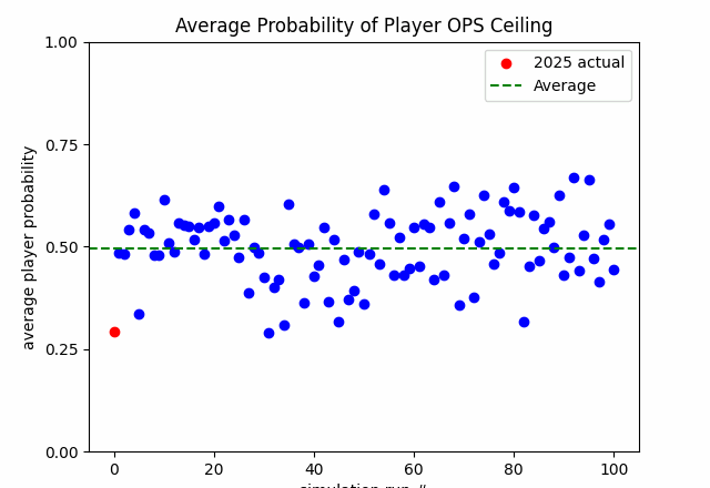
In total, we simulated 100 seasons with the results displayed below.
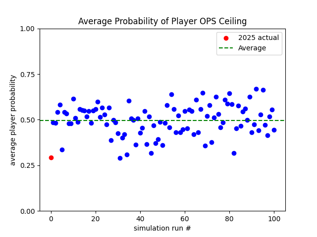
The long term average of the averages is also 50%. This makes intuitive sense. If we had to make an educated guess, we would expect that players would perform around their average…which would produce an average result in aggregate. However, there is clearly variation around the mean. As stated earlier, governed by the law of statistics, multiple players might simultaneously have poor years by random chance. The reverse is true, as well: multiple players might simultaneously have great years by random chance.
Based on the above results, the 2025 performance (so far) is highly statistically unlikely. In fact, it is the second most unlikely result in the dataset (100 simulated seasons and the 2025 partial season). Only one simulated season had a lower probability (28.9%) of occurring (which should likely be considered a statistical tie). We can, therefore, say that 2025 performance has been what we might even deem shocking, based on this statistical approach.
Now, the probabilities are likely not perfectly calibrated due to some of the issues we raised earlier in the article (bias, noise, imperfect independence, taking averages of averages can sometimes be weird). However, despite those issues, the cardinality of results should still be instructive. That is, given the data and methodology, 2025 comparatively ranks low in probability of occurrence. Again, my goal is not to construct the perfect analysis but rather one that is useful and illustrative. I believe this work accomplishes its goal.
The slapdash code can be found here.