Being inducted into Major League Baseball’s Hall of Fame (HoF) is the highest honor a baseball player can receive. The achievement is rare; many outstanding players fall short of the necessary votes. This blog presents a machine learning model, which attained strong performance, for projecting who will achieve the game’s highest honor.
About the Data
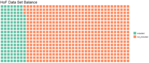
The data for this project came from the Lahman database, a respected record of historical baseball data, which I downloaded and placed in a local MySQL database. The database includes a hall of fame table, which includes year-by-year ballot results. My final data set included 716 unique players, 137 of which were inducted into the hall of fame (19%). The original data set was a bit larger (1,260 unique players, coaches, media, and executives), though for this project I opted to only focus on position players. I also removed hall of famers who were selected for historical purposes rather than voted in.
Feature Selection and Engineering
Feature selection is the process of determining what variables to use in a machine learning model, whereas feature engineering involves using existing data to develop new, informative variables. In this particular problem, almost no variable is out of the question; the baseball writers who cast their ballots can survey as much information about players as they desire. For this problem, I considered the factors voters have likely put most weight on: awards, world series titles, hits, average, etc. Some of these variables are highly correlated (e.g. hits and average), though voters probably factor in both items. For instance, a voter likely views a hitter with 2,500 hits and a .300 average different than a batter with 2,500 hits and a .280 average.
The table below displays the features used in this model. Though I am a fan of advanced statistics like WAR, such metrics have probably not guided voters’ decisions over the years.
| Variable |
|---|
| Batting Hand |
| Throwing Arm |
| Walks |
| Games Played |
| Golden Gloves |
| Hits |
| Home Runs |
| MVP Awards |
| Runs |
| RBIs |
| Stolen Bases |
| Fielding Assists |
| Fielding Put Outs |
| Errors |
| Debut Decade |
| First Year on Ballot |
| Most Frequent Position |
| Most Frequent Team |
| All-Star Appearances |
| On Base Percentage |
| Slugging Percentage |
| Batting Average |
| Postseason Batting Average |
| Postseason Games |
| World Series Wins |
| World Series Loses |
| Implicated in the Mitchell Report or Suspended for Steroids |
The inclusion of a variable to indicate whether or not a player was connected to steroids was crucial to help the model understand why, say, Barry Bonds has not been elected. To note, Gary Sheffield was not suspended or listed in the Mitchell report, so he was not labeled as “implicated”, though he has been connected to steroids in recent years. (This items was something I noticed after I had written most of this piece).
Machine Learning Approach
I applied multiple machine learning techniques within two classes of models: classification and regression. The classification models focused on predicting if someone will or will not be inducted into the hall of fame. The regression models centered on predicting the average percentage of votes a player will receive. (A player can appear on the ballot for multiple years).
Modeling Results
The results of the classification models were strong. In theory, a well-constructed model should perform well on such a problem. Hall of famers are, by definition, distinct.
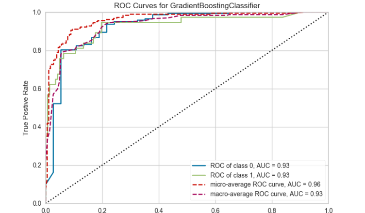
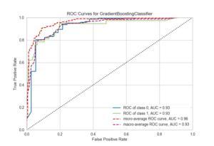
The evaluation metric employed was ROC AUC; basically, it measures the trade-off between false positives and false negatives. A score of 1.0 is the max. In this instance, a false positive occurs when the model says someone was elected but they actually were not. A false negative is the opposite, occurring when the model asserts that someone was not elected when, in fact, they were. The chart below displays the scores on the test set for different types of models. The test set is a hold-out set of data the model has not previously seen but for which we know the right answers to evaluate performance.
| Model | ROC AUC Score on Test Set |
|---|---|
| Random Forest | 0.926 |
| Extra Trees | 0.916 |
| Gradient Boosting | 0.928 |
| ADA Boost | 0.914 |
| Logistic Regression | 0.901 |
| Support Vector Machine (with polynomial kernel) | 0.898 |
| Multi-Layer Perceptron | 0.899 |
In addition, I ran models where these classifiers voted on the outcome or were stacked together in an effort to improve predictive accuracy. In a voting classifier, all models vote on the outcome of a particular case, and those results are averaged. In a stacked model, a statistical model (called a meta-estimator) makes predictions based on the patterns of predicted probabilities produced by each model.
Those scores are below, but as we can see, these more advanced models did not improve performance. To note, all voting and stacking classifiers employed the models listed in the above table.
- Voting classifier with all models voting on the outcome: 0.924
- Stacked classifier using the best tuned models and gradient boosting as the meta-estimator: 0.737
- Stacked classifier using the best tuned models and logistic regression as the meta-estimator: 0.927
- Stacked classifier using un-tuned models and gradient boosting as the meta-estimator: 0.873
- Stacked classifier using un-tuned models and logistic regression as the meta-estimator: 0.910
- Stacked classifier using a logistic regression on columns with numeric data, gradient boosting on categorical columns, and random forest as the meta-estimator: 0.723
In the above bulleted list, you might have noticed the terms “tuned” and “un-tuned”. Machine learning models have hyper-parameters, which are essentially knobs that can be turned to improve performance. For a stand-alone model, a data scientist almost always wants to discover the optimal combination of hyper-paramaters through a process called grid search. For stacking and voting, however, heavily-tuning models may not yield better performance. In fact, it may hinder performance. In the above example, we see that the logistic regression meta-estimator performed better with tuned models, whereas the gradient boosting meta-estimator was stronger with un-tuned models
At the end of the day, the stand-alone gradient boosting classifier had the strongest performance.
Whew! We’ve covered quite a bit of ground, but we’ve yet to review the regression results. As a reminder, the goal of the regression models was the predict the average percentage of votes a player will receive. This problem is more difficult. Instead of “yes” or “no”, the model must return a specific value.
The results of the regression models are OK but by no means outstanding. My focus was mostly on building a strong classification model, so I didn’t spend a ton of time squeezing out performance in the regression setting. The evaluation metric I used was root-mean-square error (RMSE), which essentially tells us how much the predictions differ from reality. In our case, an RMSE of 0.10 would mean that predictions are typically off by 10%.
Below are the results for the different regression models that were applied to the data set.
To note, it is a little peculiar that lasso and elastic net returned the same RSME, though I couldn’t find a bug in my code as the explanation.
| Model | RMSE on the Test Set |
|---|---|
| Ridge | 8.3% |
| Lasso | 9.3% |
| Elastic Net | 9.3% |
| Random Forest Regressor | 8.1% |
| Stochastic Gradient Descent | 8.7% |
| Gradient Boosting Regressor | 8.0% |
| Ordinary Least Squares with polynomial transformation applied to the data | 9.2% |
Feature Importance Scores for the Classification Model
One of the benefits of the gradient boosting classifier is that it produces feature importance scores. Below is a plot of the most important features. Read these as relative values. The variables with the top scores are not too surprising.
Probabilities Assigned to Current Hall of Famers
Below is a web app that explores the model’s predicted probability for each player being elected. A value of greater than 0.50 means the model believes the player is a hall of famer.
Here are some of the notable instances where the model was wrong. Full results can be explored in the app.
Notable False Positives (players the model asserted were in the HoF but are not)
- Bill Dahlen (an old-school player): 91% probability
- Steve Garvey: 81% probability
- Bob Meusel: 79% probability
- Dave Parker: 68% probability
Notable False Negatives (players the model asserted were not in the HoF but are)
- Willard Brown (played one year in the MLB but was mostly elected for outstanding Negro League play): 0.7% probability
- Jeff Bagwell: 11% probability
- Roy Campanella: 15% probability (he had a great Negro League career and had his career cut short due to an automobile accident; he is surely one of the greatest catchers of all time)
- Phil Rizutto: 33% probability
Outcome Discussion
In some of cases, our model didn’t have enough data to make an accurate prediction. For other instances, here’s the big question: Is the model’s assessment correct or are the voter’s correct? It’s likely that human biases play a role in who gets elected. Is this desirable? Should emotion play a role? Or would a model that only looks at the numbers be more fair? In the case of Jeff Bagwell and Phil Rizutto, I think the model is simply wrong. However, maybe a player like Dave Parker should really be in the Hall of Fame.
You can explore the results below. If the app is slow to load or only partially loads, please refresh the page.
Predictions for Future Players
I also leveraged this model to predict future hall of famers. Notable players are shown below.
In Closing
This was one of my favorite baseball analytics projects. I found the model results to be fascinating and to bring forth the following question: Should machine learning play a role in the actual hall of fame voting?
I’ll leave that one up for discussion. Thanks for reading.